Beautiful Soup
Does it bother anyone else to think about how we can’t completely describe complicated things? Most of us have heard of the Uncertainty principle describing that a more accurate measurement of position of a particle sacrifies the momentum accuracy. Here breadth, by principle, is sacrificed for depth. On a larger scale, we probably do not have enough compute on planet earth to describe a cold front, let alone weather, in a way that yeilds complete confidence in weather reports. Instead, we’d like to know generally if it will rain. This is us sacrificing depth, by lack of resources, for beadth.
It’s All Good… Enough
Small gusts of wind are hard enough to predict but we still have meteorologists measuring distributed pressure readings to deliver broad weather patterns. The cones and rods of the eye enable us to take in enough data to read, drive and explore. Our vocal transmitters and receivers are tuned to receive the propagation of waves through air, enough to say “Hey” and hear the reply in the same ~16kHz frequency band. In fact several of these disruptions in air are beautiful to us and people devote their lives to shaping and grooming the production of their features. I’m talking about audio engineers, musicians, producers and writers. This doesn’t stop at the ear - mechanical engineers study the characteristics of physical vibration through materials and RF (radiofrequency) engineers study the propagation of waves that require no medium, just like our eyes, but beyond our own capacity to see. What are the tools used that unite all of these seemingly disparate people?
Penny Fourier Thoughts?
When I look at a typical audio recording (can you tell me much about this image?) I just see chaos, and the same goes for a radio signal. But sometimes, on certain music players, the display is equipped with an EQ (equalizer). This contains a binned up view of different frequencies. Say you hear a large bass boom in the track, when that happens the lower ends of the EQ light up. If the EQ is adjustable you can even feel and hear the difference as you turn the knob. If these bins give us such a clear picture, could we enhance our understanding by creating smaller and smaller bins on the EQ? What if the bins were infinitely small? That is for what a French mathematician and aid to Napoleon, Joseph Fourier, laid the mathematical bedrock. He proposed that one can completely break down a (periodic) function into component sine waves, each with their own frequency. After some revisions from future mathematicians we are left with the Fourier Transform, granting our minds the intuition our ears and eyes had all along.
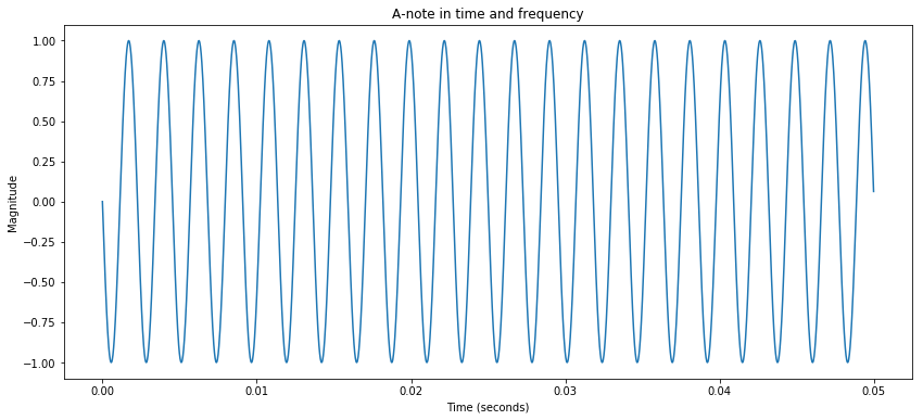
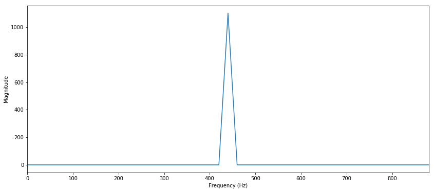
Still, there is a long way to go from this different interpretation of a signal to creating something amazing. So let’s start with the simplest wave to the ears and eyes, the sine wave. Below we have a plot of a sine wave and its corresponding Fourier Transform. FFT below means Fast Fourier Transform, it was an algorithm later developed to accelerate the DFT (Discrete Fourier Transform). What you will see and hear in various forms is an “A” note.
    import matplotlib.pyplot as plt
    import numpy as np
    # import winsound # if you are on windows

    two_pi = 2 * np.pi
    phase = np.pi/2
    frequency = 440 # "A" note in Hz
    duration_ms = 50 # miliseconds
    snr_level_db = 0
    duration_s = duration_ms/1000.0
    sample_rate = 44.1 * 1000  # Hz or samples/second
    fig_size = (14,6)

    # Beeeeep
    # winsound.Beep(frequency, duration_ms) # Beep(frequency in hz, duration in ms)

    def createCosineAudioSignal(freq, duration_s, sample_rate):
        two_pi = 2 * np.pi
        x_samples = range(int(duration_s*sample_rate))
        x_time = [(float(x_sample) / float(sample_rate)) for x_sample in x_samples]
        cosine_signal = np.cos([two_pi * frequency * time_el + phase for time_el in x_time])
        return (cosine_signal, x_samples, x_time)


    def computeFourierTransformOfSingal(signal_amplitudes, x_samples, sample_rate_hz):
        fft_signal = np.fft.fft(signal_amplitudes)
        fft_freq = np.fft.fftfreq(len(x_samples), d=(1/sample_rate_hz))
        return(fft_signal, fft_freq)

    x_samples = range(int(duration_s*sample_rate))
    x_time = [(float(x_sample) / float(sample_rate)) for x_sample in x_samples]
    (y_0, x_samples, x_time) = createCosineAudioSignal(frequency, duration_s, sample_rate)

    plt.figure(figsize=fig_size)
    plt.plot(x_time, y_0)
    plt.title('A-note in time and frequency')
    plt.xlabel('Time (seconds)')
    plt.ylabel('Magnitude')
    plt.show()

    sp = np.fft.fft(y_0)
    freq = np.fft.fftfreq(len(x_samples), d=(1/sample_rate))
    plt.figure(figsize=fig_size)
    plt.plot(freq[:int(len(freq)/2)], abs(sp[:int(len(freq)/2)]))
    plt.xlabel("Frequency (Hz)")
    plt.ylabel("Magnitude")
    plt.xlim(xmax=2*frequency, xmin = 0)
    plt.show()


Feel free to adjust the frequency, amplitude and duration to kick the tires. As you can see the frequency signal energy can be mostly found at the generating frequency. This I attribute to the imperfections of the discrete domain which could have its own post. Also, you can rest assured about negative frequencies (not shown here). If the original signal is real (and the sine wave is real… whew) there should be a symmetrical graph about 0 Hz. Think of it like turning a wheel in a different direction (more info here).
At this point it is safe to say that we can design an algorithm to bin the frequencies up and infer the signal from an input sine wave. Essentially wherever there is more energy in the frequency plot is where we most likely to find the frequency of our original wave. Our machine can listen to a perfect beep and tell us what note it is. Great. Now, what if we recorded a guitar plucking an A note? What if a truck is going by in the background of that recording? How does our methodology hold up when we start approaching the looming real world? Can we generate audio that sounds like the real world? I hope to seek the answers to some of these questions in later posts.
    min_freq = 16.35
    max_freq = 32.70

    note_to_freq = {
        "C" : 16.35,
        "Cshp_Dflt" : 17.32,
        "D" : 18.35,
        "Dshp_Eflt" : 19.45,
        "E" : 20.60,
        "F" : 21.83,
        "Fshp_Gflt" : 23.12,
        "G" : 24.50,
        "Gshp_Aflt" : 25.96,
        "A" : 27.50,
        "Ashp_Bflt" : 29.14,
        "B" : 30.87
        # "C1" : 32.70
    }

    freq_to_note = {val:key for key, val in note_to_freq.items()}
    base_freq_arr = [val for key, val in note_to_freq.items()]
    freq_arr = [val*(2**mult) for mult in range(7) for key, val in note_to_freq.items()]

    def getHighestEnergyFreq(amp_list, freq_list, verbosity=0):
        # We only care about positive frequencies which are the first half
        amp_freq_list = zip(abs(amp_list[:int(len(freq)/2)]), freq_list[:int(len(freq)/2)])

        # Get max freq
        max_amp_freq = (0,0)
        for amp_freq in amp_freq_list:
            if amp_freq[0] > max_amp_freq[0]:
                max_amp_freq = amp_freq

        if verbosity > 0:
            print("Frequncy with most amplitude: " + str(max_amp_freq[1]))

        return max_amp_freq[1]

    def getBaseFreqFromSingalFreq(starting_frequency, base_freq_arr, verbosity=0):
        """reduce the frequency to base frequency"""
        target_base_freq = starting_frequency
        while target_base_freq > base_freq_arr[len(base_freq_arr) - 1]:
            target_base_freq = target_base_freq / 2

        if verbosity > 0:
            print("Base Frequeuncy: " + str(target_base_freq))

        return target_base_freq

    def takeClosest(myList, myNumber):
        from bisect import bisect_left

        pos = bisect_left(myList, myNumber)
        if pos == 0:
            return myList[0]
        if pos == len(myList):
            return myList[-1]
        before = myList[pos - 1]
        after = myList[pos]
        if after - myNumber < myNumber - before:
            return after
        else:
            return before

    sp_highest_freq = getHighestEnergyFreq(sp, freq, verbosity=1)
    closest_freq = takeClosest(base_freq_arr, getBaseFreqFromSingalFreq(sp_highest_freq, base_freq_arr, verbosity=1))
    print("Closest Note Frequency to Base Freq: " + str(closest_freq))
    print("Determined Note: " + freq_to_note[closest_freq])
Frequncy with most amplitude: 440.0
Base Frequeuncy: 27.5
Closest Note Frequency to Base Freq: 27.5
Determined Note: A
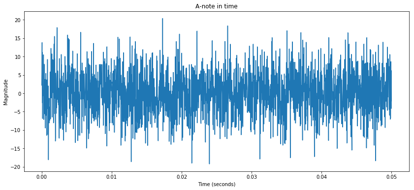
Now, I was kind of stuck back there. We can very clearly see in the Frequency plot where the peak frequency is. How can we programatically look at that and say “A”? One easy way that came to mind is to select the frequency with the maximum amplitude. This works for now, as seen above. When the picture looks that clear we could have done things such as count the y = 0 axis crossings of the signal over time, but take a look below and you’ll see that time-domain (signals where the independant variable is time) visual guessing of the frequency will not work out in high noise situations.
    def addAwgNoiseToSignal(input_discr_signal, snr_dB):
        """Calculates signal power and generates additive white gaussian noise to match SNR param"""
        sigp_dB = 10 * (np.log10(np.linalg.norm(input_discr_signal,2))**2) /\
                             len(input_discr_signal)
        noisep_dB = sigp_dB - snr_dB
        noisep = 10**(noisep_dB/10)
        noise = np.sqrt(noisep)*np.random.randn(len(input_discr_signal))
        return [sig + noise for (sig,noise) in zip(input_discr_signal, noise)]


    # Construct a new signal based off y_0 but with added noise to match the snr
    y_1 = addAwgNoiseToSignal(y_0, -15)

    plt.figure(figsize=fig_size)
    plt.plot(x_time, y_1)
    plt.title('A-note in time')
    plt.xlabel('Time (seconds)')
    plt.ylabel('Magnitude')
    plt.show()

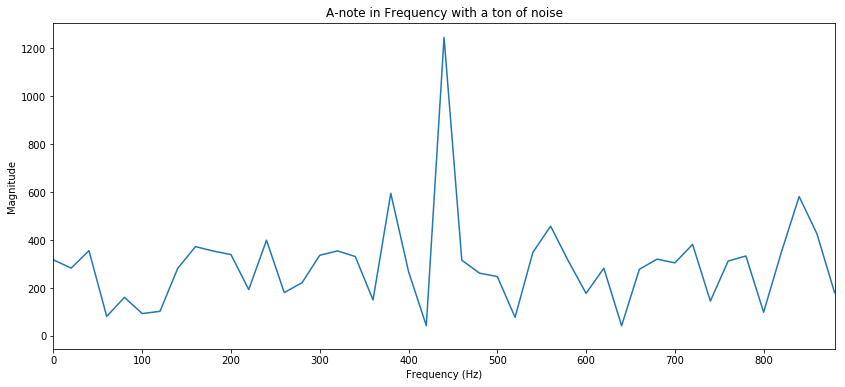
We took the same signal and just garbagized it. Now, this is a lot more noise than we would typically see in an audio setting because our noise is now twenty times larger than our signal. Do you think we’ll be able to see the signal using a fourier transform?
    (F_y_1, freq) = computeFourierTransformOfSingal(y_1, x_samples, sample_rate)

    Fy1_highest_freq = getHighestEnergyFreq(F_y_1, freq, verbosity=1)
    closest_freq = takeClosest(base_freq_arr, getBaseFreqFromSingalFreq(Fy1_highest_freq, base_freq_arr, verbosity=1))
    print("Closest Frequency to Base Freq: " + str(closest_freq))
    print("Determined Note: " + freq_to_note[closest_freq])

    plt.figure(figsize=fig_size)
    plt.plot(freq[:int(len(freq)/2)], abs(F_y_1[:int(len(freq)/2)]))
    plt.title('A-note in Frequency with a ton of noise')
    plt.xlabel("Frequency (Hz)")
    plt.ylabel("Magnitude")
    plt.xlim(xmax=2*frequency, xmin = 0)
    plt.show()
Frequncy with most amplitude: 440.0
Base Frequeuncy: 27.5
Closest Frequency to Base Freq: 27.5
Determined Note: A

How could this be? The real reason is that when we add “white” noise, we are adding noise enery that is distributed across the frequency spectrum. So even though the signal is 20 times weaker than the noise, if we know where to look, we will find the signal in an even (white) noise distribution. Nosie isn’t always white and sometimes noise can look a lot like our signal of interest. And that is someting we can explore at another time.